


Financial Accounting Ratios
Financial Accounting Ratios are important business performance indicators taken from two or more numerical results usually found within Financial Statements.
Below is a summary of the most common financial ratios along with an easy introduction on how to calculate them and how to interpret their results.

Important: Always consult an accountant before making or delaying any decisions.
Financial Accounting Ratios will be used by anyone requiring clarification as to the financial state of your business.
They also provide valuable insight into how your business is performing and will enable you to make the right next moves.
Understanding and then applying these ratios are also important when developing and confirming the viability of a business venture and assessing how feasible a business plan is when applying for loans or sourcing investment.
The figures presented within the working examples below are provided only to illustrate procedures for producing Financial Accounting Ratios and do not in any way represent or suggest assessment of performance.
There are broadly two types of Accounting Ratio
Financial Accounting Ratios consider the performance of the business by taking information from the Financial Statements of the business.
These statements are the Balance Sheet, the Income Statement and Cash Flow Statement.
This information is therefore the financial results of a business after a period of time: usually at the end of each financial year.
Management Accounting Ratios are important tools to aid the real-time management of the business during the on-going period of operation between financial results.
Here we consider Financial Accounting Ratios.
Get good at knowing the financial state of your business
You need to be familiar with the formulas below and know how to interpret and understand the variables that created them.
You don’t have to remember their construction. Just use them regularly and simply come back to this page when you need a reminder.
Gaining perspective on the ratios you see
Ratios can provide additional insight and perspective when compared to points of reference.
Points of reference can be external comparisons such as industry or competition data or internal such as your own forecasts, requirements, expectations and previous periods of performance.
Remember that ratios only provide a snap shot of the business. This is particularly so for information taken from the Balance Sheet – which by definition is a financial summary of the business taken at a particular moment in time; rather than a summary of a performance over a period of time as found with the Income Statement.
Below is a simple introduction to typical Financial Accounting Ratios.
Use the Quick Find below to click and see the ratio you are interested in.
QUICK FIND – Financial Accounting Ratios
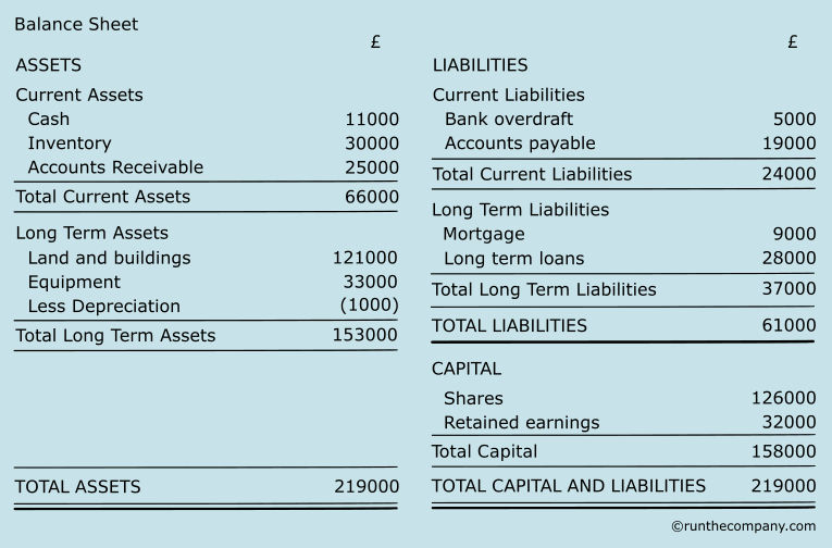
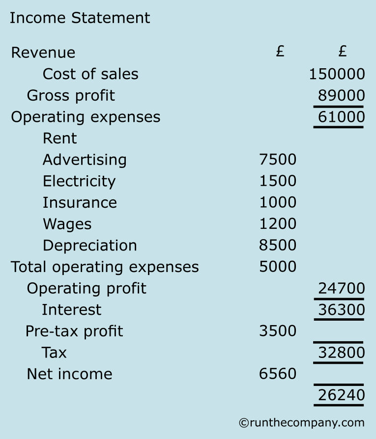
To aid comprehension, these example ratios mostly feed off the Balance Sheet and Income Statement presented below.
To be accurate, some information such as average receivables, average payables, credit sales and credit purchases require information from your accounts. Your accounting software should deliver these reports relatively easily.
Example Balance Sheet and Income Statement
Profitability
Is your business generating enough profit?
Gross Profit Margin Ratio
Purpose: Provides the percentage of Gross Profit return from Revenue after Cost of Sales have been deducted.
The result is presented as a percentage.
———————- x 100
Revenue
or in words:
Gross Profit divided by Revenue then multiplied by 100 = Gross Profit Margin percentage
Data sources:
Income Statement (Gross Profit)
——————————————————— x 100
Income Statement (Revenue)
Application example:
Gross Profit (Income Statement) = £61,000
Revenue (Income Statement) = £150,000
Application to ratio:
£61,000
—————– x 100 = 40.67%
£150,000
or in words:
£61,000 divided by £150,000 then multiplied by 100 = 40.67%
Operating Profit Margin Ratio
Purpose: Provides the percentage of Operating Profit returned from Revenue. Operating Profit Margin does not assess the quantity of sales but measures the efficiency of the business to sale at a price and manage the costs that enabled those sales.
The Operating Profit Margin Ratio therefore assesses profit before cost of finance or tax is paid. This ratio therefore considers the trading efficiency of the business and not the ability of directors to source and manage efficient finance or how effective the government is in keeping tax low.
Operating Profit can also be referred to as EBIT (Earnings Before Interest and Tax).
The result is presented as a percentage.
before interest and tax
—————————————– x 100
Revenue
or in words:
Operating Profit before interest and tax divided by Revenue then multiplied by 100 = Operating Profit Margin percentage
Data sources:
Income Statement
(Operating Profit before interest and tax)
———————————————————————-
Income Statement (Revenue)
Application example:
Operating Profit (Income Statement) = £36,300
Revenue (Income Statement) = £150,000
Application to ratio:
£36,300
————— x 100 = 24.20%
£150,000
or in words:
£36,300 divided by £150,000 then multiplied by 100 = 24.20%
The accounting gymnastics of ratios
You will likely discover various versions of some ratios out there. These merely take different routes to the same conclusions. Some also choose either percentage or decimal interpretations.
Unless you are studying to be an accountant then simply choose the ratio that best delivers the clarification and insight you require.
Return on Capital Employed (ROCE)
Purpose: Provides the percentage Operating Profit return on Capital Employed. This helps us to determine just how effective capital has been used to generate the Operating Profit.
The result is presented as a percentage.
before interest and tax
—————————————- x 100
Capital Employed
or in words:
Operating Profit divided by Capital Employed then multiplied by 100 = ROCE %
The figure for Capital Employed is constructed from information taken from the Balance Sheet.
Calculating the ROCE Ratio is therefore achieved in two steps.
Step 1: Calculate Capital Employed
Total Assets – Total Current Liabilities = Capital Employed
Data sources:
Balance Sheet (Total Assets) – Balance Sheet (Total Current liabilities) = Capital Employed
Application example:
Total Assets (Balance Sheet) = £219,000
Total Current Liabilities (Balance Sheet) = £24,000
£219,000 – £24,000 = £195,000
Capital Employed is therefore £195,000.
Step 2: Calculate ROCE
Operating Profit before interest and tax
——————————————————————– x 100
Capital Employed
Data sources:
Income Statement (Net Operating Profit)
——————————————————————- x 100
Calculation in Step 1 (Capital Employed)
Application example:
Operating Profit (Income Statement) = £36,300
Capital Employed = £195,000
£36,300
—————— x 100 = 18.62%
£195,000
or in words:
£36,300 divided by £195,000 then multiplied by 100 = 18.62%
Achieving a better percentage return on capital employed depends on improving efficiency (lower costs for the same or greater corresponding revenue) in relation to the size of the business.
Asset Turnover Ratio
Purpose: Provides the ratio of sales in relation to the size of the business. The higher the number, the better.
The result is presented as a decimal number.
————————————
Average Total Assets
or in words:
Revenue divided by Average Total Assets = Asset Turnover Ratio number
Because we use Average Total Assets, creating the Asset Turnover Ratio is done in two steps.
Step 1: Calculate Average Total Assets for the period
To find Average Total Assets you take the Total Assets from the Balance Sheet for the beginning of the period (typically from one year ago) and add the Total Assets at the end of the period (typically from the current Balance Sheet) then divide by 2.
This gives you the Average Total Assets for that period.
Total Assets at the beginning of the period
+
Total Assets at the end of the period
—————————————————————-
2
= Average Total Assets for the period
or in words
Total Assets at the beginning of the period plus Total Assets at the end of the period then divide by two =
Average Total Assets for the period
Data sources:
Start of period Balance Sheet (Total Assets) + End of period Balance Sheet (Total Assets) then divide by 2 = Average Total Assets
Application example:
In this illustrative example, we take a fictional amount to represent the Start of period Total Assets then add the Total Assets from the sample Balance Sheet provided above.
Start of period Total Assets (Start of period Balance Sheet) = £191,000
End of period Total Assets (End of period Balance Sheet) = £219,000
£191,000 + £219,000 = £410,000
———————————————————— = £205,000
2
or in words
£191,000 plus £219,000 then divide by 2 = £205,000
The Average Total Assets for the period is therefore £205,000.
Now we have the Average Total Assets for the period we can move to Step 2.
Step 2: Calculate the Asset Turnover Ratio
Revenue
———————————–
Average Total Assets
Data sources:
Income Statement (Revenue)
—————————————————————————
Calculation in Step 1 (Average Total Assets)
Application example:
Revenue (Income Statement) = £150,000
Average Total Assets (Calculation in Step 1) = £205,000
£150,000
——————- = 0.73
£205,000
or in words:
£150,000 divided by £205,000 = 0.73
This means that for every £1 employed in the company during this period, £0.73 was generated in sales.
Gearing Ratios
The Gearing Ratio is a generic term for a range of Ratios designed to determine the level of financial risk to which the business is exposed.
There are several types and formats of Gearing Ratio – each considering a slightly different aspect of gearing.
Below is one of the most common of these Ratios called the Debt to Equity Ratio.
Debt to Equity Ratio (D/E Ratio)
Purpose: Determines the amount of shareholder (owner) equity available to fulfil outstanding debt.
The result is presented as a decimal number or a percentage.
Debt to Equity Ratio as a decimal number:
————————————————–
Shareholders Equity
or in words:
Total Long Term Liabilities divided by Shareholders Equity = Debt to Equity Ratio
Debt to Equity Ratio as a percentage:
————————————————– x 100
Shareholders Equity
or in words:
Total Long Term Liabilities divided by Shareholders Equity then multiplied by 100 = Debt to Equity Ratio %
The Ratio is arrived at in two steps.
Total Long Term Liabilities can be found on the Balance Sheet.
Shareholders Equity can also be found on the Balance Sheet but may sometimes require a simple calculation to confirm the amount. The simple calculation in Step 1 below confirms that all is good.
Step 1: Calculate the amount of Shareholders Equity
Total Assets – Total Liabilities = Shareholders Equity
Data sources:
Balance Sheet (Total Assets) – Balance Sheet (Total Liabilities) = Shareholders Equity
Application example:
Total Assets (Balance Sheet) = £219,000
Total Liabilities (Balance Sheet) = £61,000
£219,000 – £61,000 = £158,000
or in words
£219,000 minus £61,000 provides £158,000 of Shareholders Equity.
Step 2: Calculate the Debt to Equity Ratio
As a decimal number:
Total Long Term Liabilities
———————————————–
Shareholders Equity
Application example:
Total Long Term Liabilities = £37,000
Shareholders Equity = £158,000
Application of ratio:
£37,000
——————- = 0.23
£158,000
or in words:
£37,000 divided by £158,000 = 0.23
which means
For every £100 of shareholder equity in the business there is £23 of debt.
As a percentage:
£37,000
——————- x 100 = 23%
£158,000
Interpretation:
The higher the Gearing Ratio number, the more that long-term capital within the business is provided by debt and therefore the higher is the risk.
However, there are many well-respected and famous companies operating on high D/E Ratios so what is an acceptable risk very much depends on the industry and circumstance.
Determining what is the right Debt to Equity Ratio for you depends on your perception of risk, the strategy and circumstances of your business, what you are attempting to achieve and the opinions of existing and potential investors and lenders.
What is important is clarity and perspective and that means comparing your existing and potential Debt to Equity Ratio to points of reference.
A low Debt to Equity Ratio might suggest lack of ambition, opportunities being missed and unfulfilled potential.
However, a low Debt to Equity Ratio and a defined opportunity requiring investment is a good place to be and is what investors and entrepreneurs like to find.
Typical ways to reduce the Debt to Equity Ratio.
- Increase revenue and therefore profit.
- Increase equity in the business through shares.
- Pay off some long-term debt.
- Convert lenders to shareholders.
Interest Coverage Ratio
Purpose: Provides a ratio between the ability to service debt (interest or financial charges) and the profit generated by the business to continue paying those charges.
The result is presented as a decimal number ratio.
before interest and tax
—————————————-
Interest charges
or in words:
Operating profit divided by Interest Charges = Interest Coverage Ratio
Data sources:
Income Statement (Operating profit)
———————————————————–
Income Statement (Interest charges)
Note: Profit before interest and tax is sometimes referred to as EBIT (Earnings Before Interest and Tax).
Application example:
Operating Profit (Income Statement) = £36,300
Interest charges (Income Statement) = £3,500
Application to ratio:
£36,300
—————– = 10.37
£3,500
Interpretation:
The higher the resulting number, the lower the risk. Although a perceptively high number may indicate the business is in a state of unrealised opportunity due to not optimising potential debt to instigate projects and make more profit.
Know that a high ratio only suggests the need for further examination. There are many more variables to consider before seeing a high number as nothing more than an indication of a circumstance. For example, the business may be repositioning its finances for a substantive capital investment either for growth or a required reaction to big market changes or competitor activities.
The lower the number, the higher the risk. For example, the business may be vulnerable to not being able to service its debt if there is an increase in interest charges and/or a trend to lower profit due to higher costs or lower revenue. Unlike the higher number scenario mentioned above, a low number ratio is more immediate in that achieving higher profit through increased revenue and/or lower costs is obviously a hard call compared to sitting on the high number ratio mentioned above.
A number closer to 1 indicates substantive risk.
This means the business is vulnerable to a downturn in the market, higher costs or higher financial costs due to such as an increase in interest rates.
Liquidity
How capable is the business in paying its debts in the short term?
In other words, what is the amount of cash available to meet the short-term obligations of the business?
Working Capital or Current Ratio
Purpose: Provides a ratio relationship number between current assets and current liabilities. This ratio confirms whether or not the business may be able to fulfil its short-term liabilities.
Although comparison to industry norms can be useful, the Current Ratio is a stand alone number in that it provides a conclusive assessment as to the capability of the business to meet its short-term obligations.
Historical and forecast points of reference will nevertheless indicate progress as regards performance.
The result is presented as a decimal number.
—————————————-
Total Current Liabilities
or in words:
Total Current Assets divided by Total Current Liabilities = Current Ratio
Data sources:
Balance Sheet (Total Current Assets)
—————————————————————
Balance Sheet (Total Current Liabilities)
Application example:
Total Current Assets = £66,000
Total Current Liabilities = £24,000
£66,000
—————– = 2.75
£24,000
or in words:
£66,000 divided by £24,000 = 2.75
Typical interpretations:
- The resulting number should show a value greater than 1.
- A number greater than 1 confirms the Current Assets within your business are greater than its short-term liabilities and the business is solvent.
- A number less than 1 would mean the business is insolvent.
- A figure approaching 1 is a reason to be concerned and remedies are required.
- As a general rule of thumb, a number of just over 2 is considered healthy; although some sectors such as retail may run a lower ratio due to low stock held (due to the short life nature of items sold), low Receivables (money owed by customers) due to mainly selling for cash and higher Payables due to extended payments terms negotiated with suppliers.
- A high ratio (disproportionately high Current Assets compared to Current Liabilities) may also indicate problems; for example, too much Inventory or high level of Receivables due to customers taking too long to pay.
For a further examination of inventory see the Inventory Turnover Ratio (Days).
To assess the level of Receivables see the Accounts Receivable Days Ratio.
Limitations:
The Current Ratio is a snapshot of the business. It does not mean the ratio is good or bad at any time before or after this snapshot was taken.
Also be aware that in reality, there are Current Assets that may not easily or quickly liquefy (turn into cash) in order to pay the bills.
For example: Inventory is part of Current Assets and if this inventory is overstocked or not selling due to a market downturn then it is unlikely cash will magically spout from these dust covered widgets.
The Quick Ratio below overcomes this particular issue by extracting Inventory from the equation.
Quick Ratio (Acid Test)
Purpose: Provides a single figure ratio between Current Assets and Current Liabilities but excludes Inventory. This number confirms whether or not the business can fulfil its short-term liabilities without undertaking the task of liquefying inventory.
Inventory may not liquefy quickly (turn to cash in the bank). After all, Stock needs to first sell and then be delivered. Invoices have to be raised and the value of these items often then revert to credit with the customer (Receivables).
By taking Inventory out of the equation, the Quick Ratio therefore provides a more potent assessment regarding the capability of the business to pay its short-term debts.
The good thing about the Acid Test is that it neatly clarifies a situation by using the few variables you have some immediate control over to influence that circumstance.
– Cash you have in the bank.
– Receivables (money owed to you).
to enable
– Payables (money you owe).
The result is presented as a decimal number.
——————————————————–
Total Current Liabilities
or in words:
Total Current Assets minus Inventory then divide by Total Current Liabilities = Quick Ratio
Data sources:
Balance Sheet (Total Current Assets)
–
Balance Sheet (Inventory)
———————————————————–
Balance Sheet (Total Current liabilities)
Application example:
Total Current Assets (Balance Sheet) = £66,000
Inventory (Balance Sheet) = £30,000
Total Current Liabilities (Balance Sheet) = £24,000
Application to ratio:
£66,000 – £30,000 = £36,000
—————————————————- = 1.5
£24,000
or in words:
£66,000 minus £30,000 then divide by £24,000 = 1.5
This means the business has £1.50 of available Current Assets to pay off every £1 of debt, if required.
Interpretation:
The Quick Ratio will obviously be lower than the Current Ratio but the resulting number should still show a value greater than 1.
Inventory Turnover Ratio (Days)
Purpose: Measures the average number of days that inventory is held within the business for the time period assessed.
The lower the number, the more efficient is the business but much depends on the sector in which the business operates and relative comparison is also likely required by using points of reference.
The result is presented as a number of days.
Note that the time period assessed below is for one year (365 days); the most common use for this ratio.
————————- x 365 days
Cost of Sales
or in words:
Inventory divided by Cost of Sales then multiplied by the number of days assessed (in this case 365 representing one year).
Date sources:
Balance Sheet (Inventory)
——————————————————— x 365 days
Income Statement (Cost of sales)
Application example:
Inventory (Balance Sheet) = £30,000
Cost of sales (Income Statement) = £89,000
Days assessed = 365
Application to ratio
£30,000
—————- x 365 = 123.03 days
£89,000
or in words:
£30,000 divided by £89,000 then multiplied by 365 = 123.03 days
This means the average days inventory is held within the business before being sold is 123 days.
Interpretations:
Reducing the Inventory Days figure is a measurement of improving efficiency but should be compared to internal and external points of reference for perspective.
Be aware that in striving for an ever reducing Inventory Days figure will at some point involve an increasing dependence on a Just in Time stock management policy.
There is a correlation between increasing the level of Just in Time and increased risk. Squeezing the cushion of time out of your logistics is good from a financial performance perspective but it does increase the risk of problems when supplies are delayed for even the most minor of reasons.
Deliveries delayed beyond the procurement schedule will affect production and increase the potential for late deliveries to customers (meaning delayed invoicing) or being out of stock when a customer is ordering (losing sales revenue) and potentially resulting in a damaged reputation (losing market share to competition).
In other words, there is an optimum point for Inventory Days depending on the supply chain of your industry and the simple practicalities of your logistics and market.
Limitations:
Note that Inventory Days is an assessment from a monetary value perspective and not of individual physical items.
For example, this analysis will not take relative account of that big fat six foot square package taking up room in your warehouse if its value does not reflect its physical size.
Nevertheless, that big fat thing and perhaps many more like it could be taking up space; space that could be used for higher turnover and therefore potentially more profit generating alternatives.
The Inventory Turnover Ratio is therefore crucial to assessing the performance of stock throughput from a generic and concluding financial perspective but additional measures of performance are also required when seeking optimum stock management.
Accounts Receivable Days Ratio
Purpose: Determines the average number of days customers are taking to pay.
Accounts Receivable is the outstanding amount of money owed by customers.
The result is presented as a number of days.
Note that for this ratio, we should only include Credit Sales as the inclusion of cash sales will disrupt the analysis and disguise the extent to which credit sales might be a problem.
Where the Current Ratio and Quick Ratio (Acid Test) are high then a clue to the issue may be provided by this ratio.
Note that the time period assessed below is for one year (365 days); the most common use for this ratio.
————————————————— x 365 days
Total Credit Sales
or in words:
Average Accounts Receivable divided by Total Credit Sales then multiplied by 365 = Average collection days
We use an Average Accounts Receivable figure for the period being considered.
This means the analysis is done in three steps.
Step 1: Calculate the Average Accounts Receivable for the period
To find Average Accounts Receivable you take the Accounts Receivable figure from the Balance Sheet representing the beginning of the period (typically from the previous year) and add the Accounts Receivable at the end of the period (typically from the current Balance Sheet) then divide by two. This gives you the Average Accounts Receivable for that period.
Accounts Receivable at the beginning of the period
+
Accounts Receivable at the end of the period
——————————————————————————
2
= Average Accounts Receivable for the period
or in words
Accounts Receivable at the beginning of the period plus Accounts Receivable at the end of the period then divide by two = Average Accounts Receivable for the period
Data sources:
Start of period Balance Sheet (Accounts Receivable) + End of period Balance Sheet (Accounts Receivable then divide by 2 = Average Accounts Receivable
Application example:
For this illustrative example, we take a fictional amount to represent the Start of period Accounts Receivable then add the Accounts Receivable from the sample Balance Sheet provided at the top of this page.
Start of period Accounts Receivable (Start of period Balance Sheet)= £20,000
End of period Accounts Receivable (End of period Balance Sheet) = £25,000
this provides
£20,000 + £25,000 = £45,000
Then divide by 2:
£45,000 divided by 2 = £22,500
The average Accounts Receivable for the period is £22,500.
Now we have the Average Accounts Receivable for the period we can move to Step 2.
Step 2: Determine the Total Credit Sales during the period
Unless all sales were Credit Sales (no cash sales) during the year then using the Revenue figure from the Income Statement for this ratio could be deceptive.
To achieve an accurate figure for Total Credit Sales for the period, you would have to run a report in your accounting software; then use that figure in the bottom half of the formula. This is shown in bold in the formula below.
Average Accounts Receivable
————————————————- x 365 days
Total Credit Sales
Application example:
In the application example below, we have assumed that all Revenue in the Income Statement example at the top of this page was achieved through credit sales only.
Total Credit Sales for this period = £150,000
We now have the following information required for Step three:
Average Accounts Receivable = £22,500
Total Credit Sales = £150,000
Step 3: Calculate the Accounts Receivable days
Average Accounts Receivable
————————————————- x 365 days
Credit Sales
Application example:
Average Accounts Receivable – taken from the above Step 1 procedure above = £22,500
Total Credit Sales – taken from the above Step 2 procedure above = £150,000
Number of days (year) = 365
Application to ratio:
£22,500
—————— x 365 = 54.75 days
£150,000
or in words:
£22,500 divided by £150,000 then multiplied by 365 = 54.75 days
This means the credit customers for this business are taking an average of 55 days to pay their invoices.
Typical interpretations:
The number of days customers take to pay is determined by two factors.
• Credit terms provided to customers.
• The extent to which customers pay on time.
From a cash efficiency perspective, this number should ideally be lower or at least equal to the Accounts Payable Days Ratio (see below).
The Accounts Receivable Days Ratio should be compared to the actual credit control policy of the business.
The credit control policy can then be confirmed, reviewed or tightened depending on the findings.
For example, if the credit control objective for the business was to sell on 30 day credit terms and this ratio returned as 90 days then this would indicate a problem with late payers.
Note though that the returning figure is an average return and therefore further analysis is required. The business may have many customers paying on time but one or a few large customers paying late.
In terms of further investigation and potential action, the following typical variables may be at play:
- The number of customers paying late or trend (there may be increasing cash pressure in your market sector).
- Sizeable debt customers are being allowed (sales terms may be liberal in order to win the business due to over-geared internal sales objectives or pressure from competition).
- One or a few customers know how important they are to you and are using this advantage by paying late.
- One a more larger customers may have cash flow issues due to their internal circumstances and management decisions. This also indicates increased risk to your business.
The Accounts Receivable Days Ratio should also be compared to that expected for your industry. It may not be realistic to demand 30 days credit from customers if your competition is offering 90 days.
Such practices are usually due to cashflow necessity caused by the financial logistics within sectors or trends brought about by competitors offering more favourable terms to win business.
Comparing this ratio to historical data will help clarify credit control performance of the business over time.
Alternatively, a trend down can mean improving credit control.
Limitations:
Be aware that this ratio is a snapshot and likely the result of the end of year financial statements. Receivables may be disproportionately high or low at end of year.
Accounts Payable Days Ratio
Purpose: Determines the average number of days the business is taking to pay its suppliers.
The result is presented as a number of days.
Accounts Payable is the money owed to all suppliers.
Note that the time period assessed below is for one year (365 days); the most common use for this ratio.
———————————————- x 365
Total Credit Purchases
or in words:
Average Accounts Payable divided by Total Credit Purchases then multiplied by 365 = Average Payment Period (payable days)
We therefore use an Average Accounts Payablee figure for the period being considered and a figure for purchases made on credit (Credit Purchases).
This means the analysis is done in three steps.
Step 1: Calculate the Average Accounts Payable for the period
To find Average Accounts Payable you take the Accounts Payable figure from the Balance Sheet representing the beginning of the period (typically from the previous year) and add the Accounts Payable at the end of the period (typically from the current Balance Sheet) then divide by two. This gives you the Average Accounts Payable for that period.
Accounts Payable at the beginning of the period
+
Accounts Payable at the end of the period
————————————————————————–
2
= Average Accounts Payable for the period
Data sources:
Start of period Balance Sheet (Accounts Payable) + End of period Balance Sheet (Accounts Payable then divide by 2 = Average Accounts Payable
Application example:
For this particular example, we take a fictional amount of £17,000 to represent the Start of period Accounts Payable then add the Accounts Payable £19,000 from the sample Balance Sheet provided at the top of this page.
Start of period Accounts Payable (Start of period Balance Sheet)= £17,000
End of period Accounts Payable (End of period Balance Sheet) = £19,000
this provides
£17,000 + £19,000 = £36,000
Then divide by 2:
£36,000 divided by 2 = £18,000
The average Accounts payable for the period is £18,000.
Now we have the average Accounts Payable for the period we can move to Step 2.
Step 2: Determine the Total Credit Purchases during the period
Note that Total Credit Purchases should only include purchases made on credit as the inclusion of cash purchases will disrupt the analysis.
To achieve an accurate figure for Total Credit Purchases for the period, you will have to run a report in your accounting software; then use that figure for the bottom half of the formula.
This is shown in bold in the formula below.
Average Accounts Payable
——————————————— x 365
Total Credit Purchases
In the illustrative example below, we have assumed that all Cost of Sales and Expenses in the Income Statement example at the top of this page were incurred through credit purchases only.
Application example:
Total Credit Purchases for this period = £100,200
We now have the following information required for Step three:
Average Accounts Payable = £18,000
Total Credit Purchases = £100,200
Step 3: Calculate the Accounts Payable days
Average Accounts Payable
———————————————- x 365
Total Credit Purchases
Application example:
Average Accounts Payable – taken from the above Step 1 procedure = £18,000
Total Credit Purchases – taken from the above Step 2 procedure = £100,200
Number of days (year) = 365
£18,000
—————— x 365 = 65.57 days
£100,200
or in words:
£18,000 divided by £100,200 then multiplied by 365 = 65.57 days
This means the business is taking an average of 66 days to pay its suppliers.
Typical Interpretations:
The number of days we take to pay suppliers is determined by two factors.
• Credit terms negotiated with suppliers.
• The extent to which we adhere to those credit terms.
From a cash efficiency perspective, this Payable Days Ratio should ideally be higher or at least equal to the Accounts Receivable Days Ratio (see above).
Both Ratios should be compared to the actual credit control policy of the business.
Be aware that there is a limit to which you can push the number of days you take to pay the bills. Striving for an ever increasing Accounts Payable Days Ratio and therefore a more favourable ratio between Payable Days and Receivable Days can increase the risk of legal proceedings from frustrated suppliers and a potential negative impact on credit rating.
If you are squeezing supplier cashflow, then they may allow for this in their pricing or discount structure; or reduce the depth of service available to you. Remember, the money has to come from somewhere.
Having a reputation for being a bad payer may also mean you only end up doing business with less competitive suppliers (those less able and therefore more desperate and willing to tolerate a slow paying customer). It might even compromise your frontend brand in the marketplace.
Getting a perspective on the Accounts Payable Days Ratio
In summary, the following two points of reference will help provide perspective.
- Compare the Accounts Payable Days Ratio to the Accounts Receivable Days Ratio (remember that you want to be cash positive).
- Industry average. For example, knowing how long your competitors take to pay will mean you can fit within the norm or offer a competitive advantage by paying faster in return for favourable service or price discounts.
Knowing how the opposing two camps behind Receivables and Payables arm wrestle will enable you to ask fundamental but insightful questions.
Why should sales be compromised due to inflexible customer credit terms that are out of sync with the market average or customers are hassled for payment because your purchasing department lazily agrees short-time credit terms with suppliers?
or
Why should good suppliers be put under pressure because our sales department weakly gives away short-time credit terms or we are overly timid of that big fat slow paying customer?